Assigning bulk RNA-seq to pseudotime
assign-bulk-to-pseudotime.Rmd
library(blase)
library(SingleCellExperiment)
library(tradeSeq)
library(slingshot)
library(scran)
library(scater)
library(BiocParallel)
library(ami)
library(patchwork)
library(reshape2)
RNGversion("3.5.0")
#> Warning in RNGkind("Mersenne-Twister", "Inversion", "Rounding"): non-uniform
#> 'Rounding' sampler used
SEED <- 7
set.seed(SEED)
N_CORES <- 4
if (ami::using_ci()) {
    N_CORES <- 2
}
Introduction
BLASE is a tool for matching bulk RNA-seq samples to the pseudotime
of a trajectory in a scRNA-seq dataset. BLASE integrates with the
Bioconductor ecosystem by integrating closely with SingleCellExperiment
objects. (BLASE can be used with Seurat objects that have been converted
using as.SingleCellExperiment.)
BLASE can be used for the following use-cases: * Identifying the progress of a bulk like RNA-seq sample through scRNA-seq reference trajectory. * Annotating scRNA-seq trajectories with reference bulk RNA-seq datasets * Correcting development rate differences in comparative RNA-seq samples.
Principle
We believe that in many trajectories that cells undergo, there will be a curve that shows the expression of some key genes. In the plot below, we can see that by looking at these three “genes” which have 2 peaks each over “pseudotime”, we can identify 6 unique states, which, as long as the genes correspond to some aspect of the trajectory, can be used to infer which stage of the trajectory a cell is currently in. This is of course a constructed example and unlikely to be exactly repeated in real life, but hopefully demonstrates the principle BLASE works on.
# Adapted from
# https://codepal.ai/code-generator/query/n4dEA6I9/plot-sine-wave-ggplot2-r
x <- seq(0, 2 * pi, length.out = 500)
gene1_expr <- 10 * (sin(x + 0.1) + 1)
gene2_expr <- 11 * (sin(x - pi) + 1)
gene3_expr <- 7 * (sin(x + pi / 2) + 1)

genes <- data.frame(gene1 = gene1_expr, gene2 = gene2_expr, gene3 = gene3_expr)
genes_melt <- melt(t(genes), varnames = c("gene", "x"))
genes_melt$x <- as.numeric(genes_melt$x)
ggplot(genes_melt, aes = aes()) +
    geom_line(aes(x = x, y = value, color = gene)) +
    geom_vline(xintercept = 0, linetype = "dashed") +
    geom_vline(xintercept = 24, linetype = "dashed") +
    geom_vline(xintercept = 181, linetype = "dashed") +
    geom_vline(xintercept = 243, linetype = "dashed") +
    geom_vline(xintercept = 315, linetype = "dashed") +
    geom_vline(xintercept = 479, linetype = "dashed") +
    geom_vline(xintercept = 500, linetype = "dashed") +
    labs(
        x = "pseudotime",
        y = "Gene Expression",
        title = "Variable Genes Over Pseudotime"
    )
#> Warning in fortify(data, ...): Arguments in `...` must be used.
#> ✖ Problematic argument:
#> • aes = aes()
#> ℹ Did you misspell an argument name?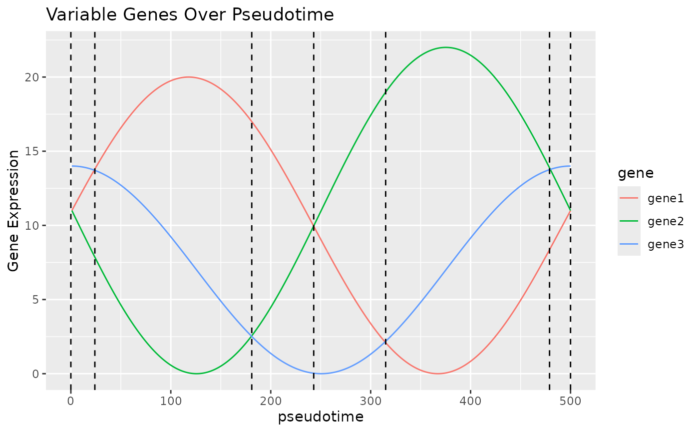
In this vignette, we will use BLASE to try to assign bulk RNA-seq samples to the pseudotime trajectory in a scRNA-seq data. We need to have the following to use Blase in this case:
- A Single Cell Experiment with pseudotime.
- A list of genes that explain the trajectory well, in this case
generated by tradeSeq’s
fitGAMandassociationTest
Installing BLASE
To install BLASE from Bioconductor:
if (!require("BiocManager", quietly = TRUE)) install.packages("BiocManager")

BiocManager::install("blase")
Setting up the Single Cell Experiment
First, let’s load a Single Cell Experiment to use the tool with, based on the tradeSeq vignette. We have added pseudotime to the object, and used tradeSeq as shown in their vignette.
data(tradeSeq_BLASE_example_sce, package = "blase")
sce <- tradeSeq_BLASE_example_sce
plotUMAP(sce, text_by = "celltype", colour_by = "celltype") +
    plotUMAP(sce, colour_by = "pseudotime") +
    patchwork::plot_layout(ncol = 1, axis_title = "collect")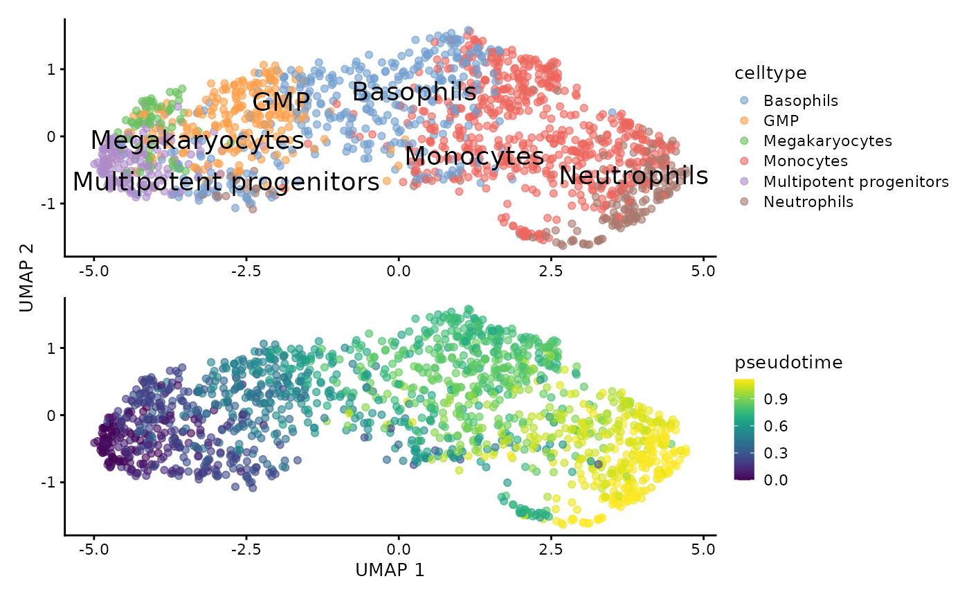
Finding the most descriptive genes with tradeSeq
Now we’ll find the genes we want to use. We select the top 200 so that we can do some parameter tuning below.
# Use consecutive for genes that change over time
assoRes <- associationTest(
    sce,
    lineages = TRUE,
    global = FALSE,
    contrastType = "consecutive"
)
genelist <- blase::get_top_n_genes(assoRes, n_genes = 200, lineage = 1)
Please note that other methods of selecting genes are available. Please see other vignettes for details.
Parameter Tuning for BLASE
When using BLASE, it can be a good idea to tune the number of genes and bins used.
- Too few genes can lead to poor fitting
- Too many genes can lead to slower execution, without any benefit, as the less informative genes still need to be checked.
- Too few bins can oversimplify the trajectory
- Too many bins can lead to too few cells being available for reliable values.
We can do this using the following commands, provided by BLASE:
res <- blase::find_best_params(
    sce,
    genelist,
    split_by = "pseudotime_range",
    pseudotime_slot = "pseudotime",
    bins_count_range = c(5, 10),
    gene_count_range = c(40, 80)
)
blase::plot_find_best_params_results(res)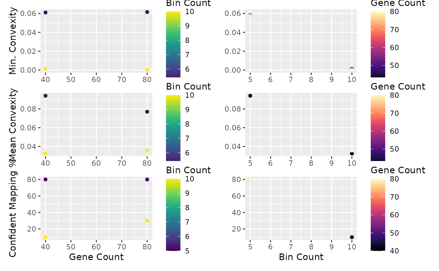
It looks like 80 genes and 10 bins will give us good specificity, but let’s double check. In a non trivial dataset, this may take some repetition. We ignore the 5 bin result because this might not be enough resolution - this depends on your dataset. In general, more bins will reduce specificity because each bin will have a more similar cell composition. In general, aim for about as many bins as you have clusters.
Inspect Bin Choice
Now we can check if this is a good fit by showing how other bins from the SC dataset map using these genes. Ideally, each bin is very specific, with a high “worst specificity”.
blase_data <- as.BlaseData(sce, pseudotime_slot = "pseudotime", n_bins = 10)
genes(blase_data) <- genelist[1:80]
evaluate_parameters(blase_data, make_plot = TRUE)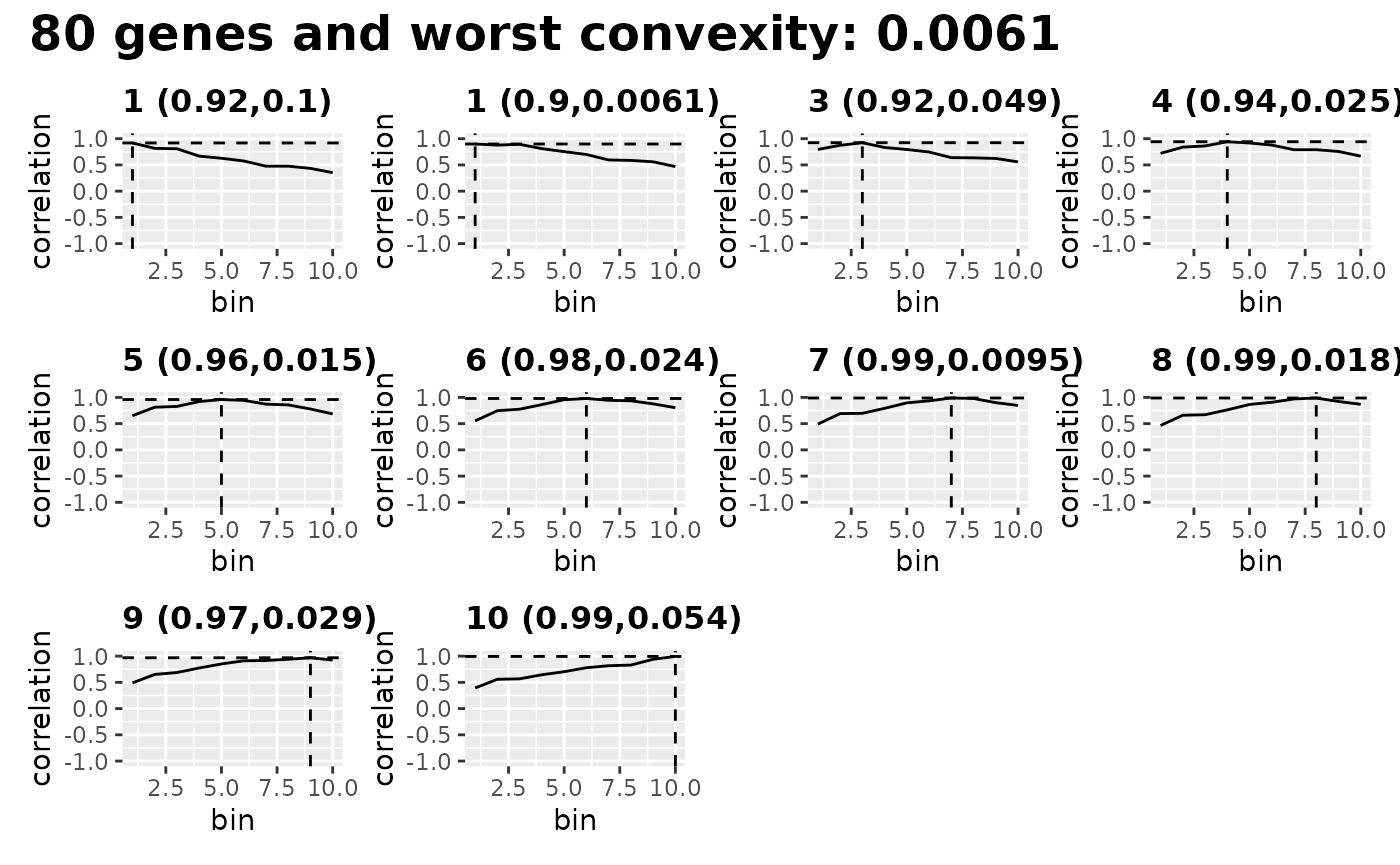
#> [1] 0.00610 0.03322 10.00000Inspect Genes Choice
We can also see how the genes change over pseudotime, by plotting expression of the top genes changing over each pseudotime bin.
evaluate_top_n_genes(blase_data)<img src=“/home/runner/work/blase/blase/docs/articles/assign-bulk-to-pseudotime_files/figure-html/evaluateTopGenes-1.png” class=“r-plt” alt=“Plot showing a the”best” genes selected for use with BLASE, according to how related their expression is to the pseudotime of the cell.” width=“700” />
Mapping Bulk Samples to SC with BLASE
If we’re happy, now we can try to map a bulk sample onto the single cell. We’ll do this by pseudobulking cell types in the SingleCellExperiment but in reality you should use a real bulk dataset. See some of our other articles for examples.
bulks_df <- DataFrame(row.names = rownames(counts(sce)))
for (type in unique(sce$celltype)) {
    bulks_df <- cbind(
        bulks_df,
        rowSums(normcounts(subset(sce, , celltype == type)))
    )
}

colnames(bulks_df) <- unique(sce$celltype)

multipotent_progenitors_result <- map_best_bin(
    blase_data, "Multipotent progenitors", bulks_df
)
multipotent_progenitors_result
#> MappingResult for 'Multipotent progenitors': best_bin=1 correlation=0.993975621190811 top_2_distance=0.07
#>   Strong Result: TRUE (next max upper  0.944742828998288 )
#>   with history for scores against 10  bins
#>   Bootstrapped with 200 iterations
basophils_result <- map_best_bin(blase_data, "Basophils", bulks_df)
basophils_result
#> MappingResult for 'Basophils': best_bin=6 correlation=0.965002344116268 top_2_distance=4e-04
#>   Strong Result: FALSE (next max upper  0.981492775379996 )
#>   with history for scores against 10  bins
#>   Bootstrapped with 200 iterations
neutrophils_result <- map_best_bin(blase_data, "Neutrophils", bulks_df)
neutrophils_result
#> MappingResult for 'Neutrophils': best_bin=10 correlation=0.990412564463197 top_2_distance=0.0676
#>   Strong Result: TRUE (next max upper  0.952775855395118 )
#>   with history for scores against 10  bins
#>   Bootstrapped with 200 iterations
We can also generate this result with map_all_best_bins,
which can also allow for parallelisation of the process for large
numbers of bulks:
map_all_best_bins(blase_data, bulks_df)
#> [[1]]
#> MappingResult for 'Multipotent progenitors': best_bin=1 correlation=0.993975621190811 top_2_distance=0.07
#>   Strong Result: TRUE (next max upper  0.947814053851206 )
#>   with history for scores against 10  bins
#>   Bootstrapped with 200 iterations
#>
#> [[2]]
#> MappingResult for 'Monocytes': best_bin=9 correlation=0.984481950304735 top_2_distance=0.0245
#>   Strong Result: FALSE (next max upper  0.979289316289433 )
#>   with history for scores against 10  bins
#>   Bootstrapped with 200 iterations
#>
#> [[3]]
#> MappingResult for 'Neutrophils': best_bin=10 correlation=0.990412564463197 top_2_distance=0.0676
#>   Strong Result: TRUE (next max upper  0.949364416717482 )
#>   with history for scores against 10  bins
#>   Bootstrapped with 200 iterations
#>
#> [[4]]
#> MappingResult for 'Basophils': best_bin=6 correlation=0.965002344116268 top_2_distance=4e-04
#>   Strong Result: FALSE (next max upper  0.982104324983582 )
#>   with history for scores against 10  bins
#>   Bootstrapped with 200 iterations
#>
#> [[5]]
#> MappingResult for 'Megakaryocytes': best_bin=3 correlation=0.833380215658697 top_2_distance=0.0102
#>   Strong Result: FALSE (next max upper  0.900887695392662 )
#>   with history for scores against 10  bins
#>   Bootstrapped with 200 iterations
#>
#> [[6]]
#> MappingResult for 'GMP': best_bin=4 correlation=0.984857008907642 top_2_distance=0.0398
#>   Strong Result: FALSE (next max upper  0.977275392228138 )
#>   with history for scores against 10  bins
#>   Bootstrapped with 200 iterations
Plotting Heatmap of Mappings
To see how well we plotted the differences between these cell types, we can plot a heatmap of all these results. The neutrophils and Erythrocytes are strongly mapped, but the GMP population doesn’t map as well.
plot_mapping_result_heatmap(list(
    multipotent_progenitors_result,
    basophils_result,
    neutrophils_result
), annotate_correlation = TRUE, text_background = TRUE)
#> Inferred correlation metric.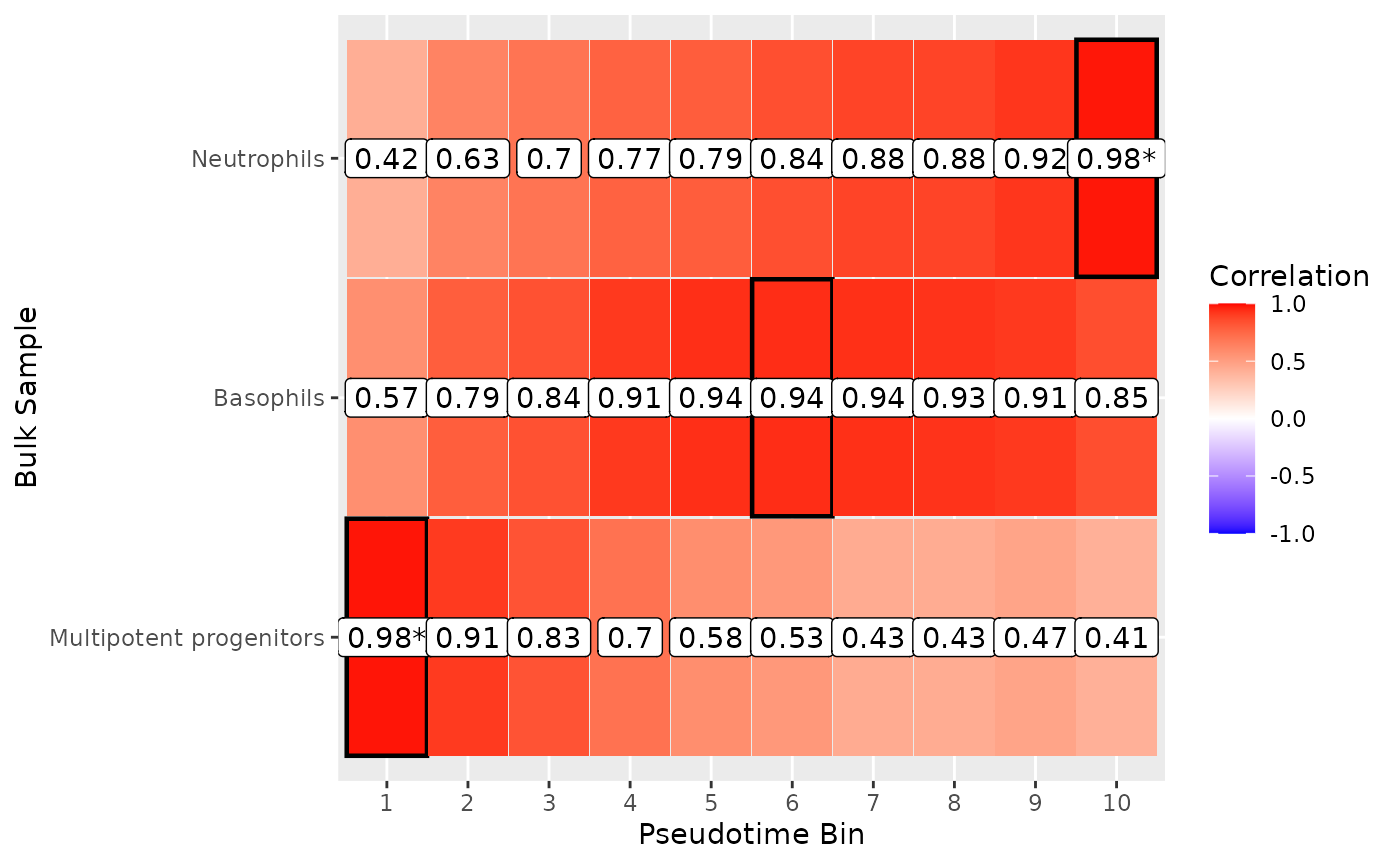
Plotting Detailed Correlation Maps
To look into the Basophils mapping, we can plot the correlation over each bin. Because the the lower boundary of the best selection (bin 3) is higher than the higher bounds of the next-best bin (bin 4), BLASE makes a strong call.
plot_mapping_result_corr(basophils_result)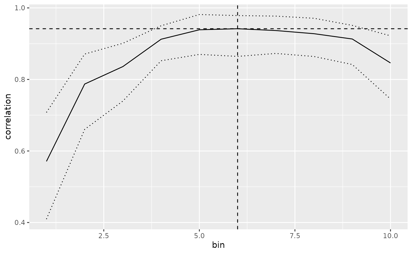
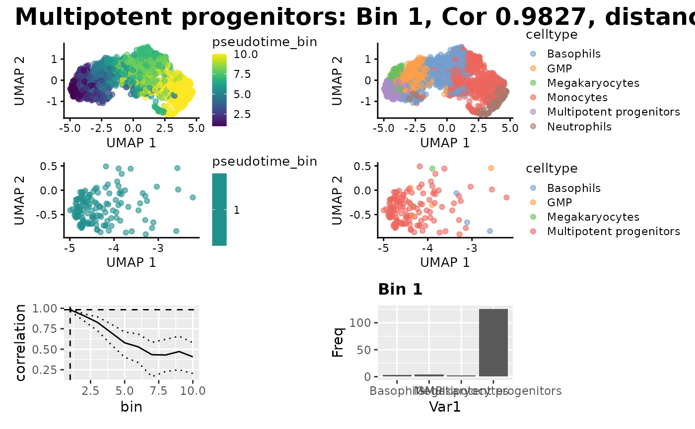
Plotting Summary Plots of Mappings
Now we can do some more detailed plotting about where the bins mapped onto the Single Cell data, and the cell type proportions we expect , but we need to add the pseudotime bins to the metadata of the SCE. We can see that the true proportions of cell types in the mapped bin do indeed map to the cell type we expect.
binned_sce <- assign_pseudotime_bins(
    sce,
    split_by = "pseudotime_range",
    n_bins = 10,
    pseudotime_slot = "pseudotime"
)
plot_mapping_result(
    binned_sce,
    multipotent_progenitors_result,
    group_by_slot = "celltype"
)
To view the bin population chart in full, use:
plot_bin_population(binned_sce, 1, group_by_slot = "celltype")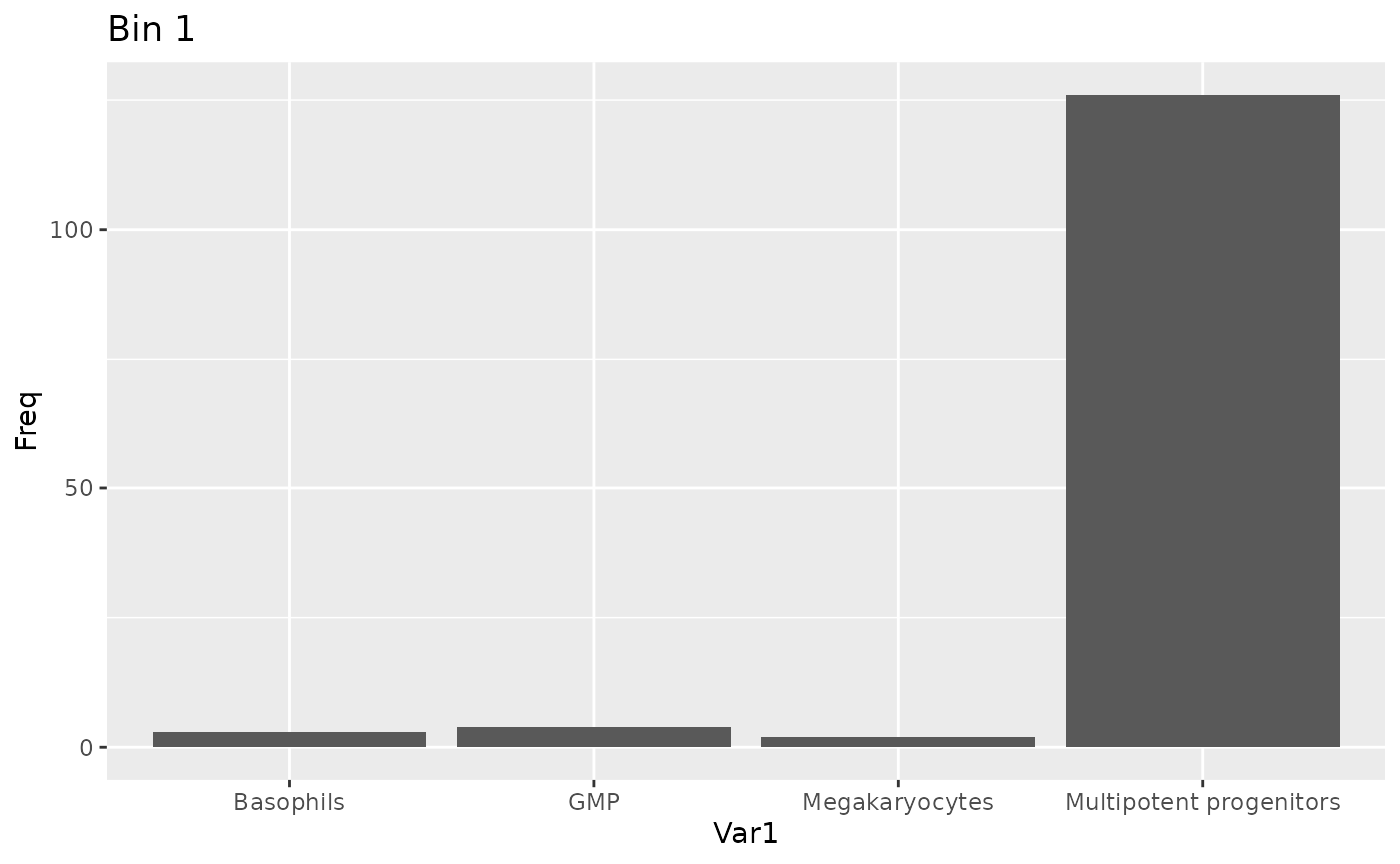
Session Info
sessionInfo()
#> R version 4.6.0 (2026-04-24)
#> Platform: x86_64-pc-linux-gnu
#> Running under: Ubuntu 24.04.4 LTS
#>
#> Matrix products: default
#> BLAS:   /usr/lib/x86_64-linux-gnu/openblas-pthread/libblas.so.3
#> LAPACK: /usr/lib/x86_64-linux-gnu/openblas-pthread/libopenblasp-r0.3.26.so;  LAPACK version 3.12.0
#>
#> Random number generation:
#>  RNG:     Mersenne-Twister
#>  Normal:  Inversion
#>  Sample:  Rounding
#>
#> locale:
#>  [1] LC_CTYPE=C.UTF-8       LC_NUMERIC=C           LC_TIME=C.UTF-8
#>  [4] LC_COLLATE=C.UTF-8     LC_MONETARY=C.UTF-8    LC_MESSAGES=C.UTF-8
#>  [7] LC_PAPER=C.UTF-8       LC_NAME=C              LC_ADDRESS=C
#> [10] LC_TELEPHONE=C         LC_MEASUREMENT=C.UTF-8 LC_IDENTIFICATION=C
#>
#> time zone: UTC
#> tzcode source: system (glibc)
#>
#> attached base packages:
#> [1] stats4    stats     graphics  grDevices utils     datasets  methods
#> [8] base
#>
#> other attached packages:
#>  [1] reshape2_1.4.5              patchwork_1.3.2
#>  [3] ami_0.2.1                   BiocParallel_1.46.0
#>  [5] scater_1.40.1               ggplot2_4.0.3
#>  [7] scran_1.40.0                scuttle_1.22.0
#>  [9] slingshot_2.20.0            TrajectoryUtils_1.20.0
#> [11] princurve_2.1.6             tradeSeq_1.26.0
#> [13] SingleCellExperiment_1.34.0 SummarizedExperiment_1.42.0
#> [15] Biobase_2.72.0              GenomicRanges_1.64.0
#> [17] Seqinfo_1.2.0               IRanges_2.46.0
#> [19] S4Vectors_0.50.1            BiocGenerics_0.58.1
#> [21] generics_0.1.4              MatrixGenerics_1.24.0
#> [23] matrixStats_1.5.0           blase_1.3.0
#> [25] BiocStyle_2.40.0
#>
#> loaded via a namespace (and not attached):
#>   [1] RcppAnnoy_0.0.23       splines_4.6.0          later_1.4.8
#>   [4] tibble_3.3.1           polyclip_1.10-7        fastDummies_1.7.6
#>   [7] lifecycle_1.0.5        edgeR_4.10.1           globals_0.19.1
#>  [10] lattice_0.22-9         MASS_7.3-65            SnowballC_0.7.1
#>  [13] magrittr_2.0.5         limma_3.68.3           plotly_4.12.0
#>  [16] sass_0.4.10            rmarkdown_2.31         jquerylib_0.1.4
#>  [19] yaml_2.3.12            metapod_1.20.0         httpuv_1.6.17
#>  [22] otel_0.2.0             Seurat_5.5.0           sctransform_0.4.3
#>  [25] spam_2.11-3            sp_2.2-1               spatstat.sparse_3.2-0
#>  [28] reticulate_1.46.0      cowplot_1.2.0          pbapply_1.7-4
#>  [31] RColorBrewer_1.1-3     abind_1.4-8            Rtsne_0.17
#>  [34] purrr_1.2.2            ggrepel_0.9.8          irlba_2.3.7
#>  [37] listenv_0.10.1         spatstat.utils_3.2-3   goftest_1.2-3
#>  [40] RSpectra_0.16-2        dqrng_0.4.1            spatstat.random_3.5-0
#>  [43] fitdistrplus_1.2-6     parallelly_1.47.0      pkgdown_2.2.0
#>  [46] codetools_0.2-20       DelayedArray_0.38.1    tidyselect_1.2.1
#>  [49] farver_2.1.2           ScaledMatrix_1.20.0    viridis_0.6.5
#>  [52] spatstat.explore_3.8-1 jsonlite_2.0.0         BiocNeighbors_2.6.0
#>  [55] progressr_0.19.0       ggridges_0.5.7         survival_3.8-6
#>  [58] systemfonts_1.3.2      tools_4.6.0            ragg_1.5.2
#>  [61] ica_1.0-3              Rcpp_1.1.1-1.1         glue_1.8.1
#>  [64] gridExtra_2.3          SparseArray_1.12.2     xfun_0.57
#>  [67] mgcv_1.9-4             dplyr_1.2.1            withr_3.0.2
#>  [70] BiocManager_1.30.27    fastmap_1.2.0          bluster_1.22.0
#>  [73] boot_1.3-32            digest_0.6.39          rsvd_1.0.5
#>  [76] R6_2.6.1               mime_0.13              textshaping_1.0.5
#>  [79] scattermore_1.2        tensor_1.5.1           spatstat.data_3.1-9
#>  [82] tidyr_1.3.2            data.table_1.18.4      httr_1.4.8
#>  [85] htmlwidgets_1.6.4      S4Arrays_1.12.0        uwot_0.2.4
#>  [88] pkgconfig_2.0.3        gtable_0.3.6           lmtest_0.9-40
#>  [91] S7_0.2.2               XVector_0.52.0         htmltools_0.5.9
#>  [94] dotCall64_1.2          bookdown_0.46          SeuratObject_5.4.0
#>  [97] scales_1.4.0           png_0.1-9              spatstat.univar_3.2-0
#> [100] knitr_1.51             nlme_3.1-169           cachem_1.1.0
#> [103] zoo_1.8-15             stringr_1.6.0          KernSmooth_2.23-26
#> [106] parallel_4.6.0         miniUI_0.1.2           vipor_0.4.7
#> [109] desc_1.4.3             pillar_1.11.1          grid_4.6.0
#> [112] vctrs_0.7.3            RANN_2.6.2             lsa_0.73.4
#> [115] promises_1.5.0         BiocSingular_1.28.0    beachmat_2.28.0
#> [118] xtable_1.8-8           cluster_2.1.8.2        beeswarm_0.4.0
#> [121] evaluate_1.0.5         locfit_1.5-9.12        cli_3.6.6
#> [124] compiler_4.6.0         rlang_1.2.0            future.apply_1.20.2
#> [127] labeling_0.4.3         plyr_1.8.9             fs_2.1.0
#> [130] ggbeeswarm_0.7.3       stringi_1.8.7          viridisLite_0.4.3
#> [133] deldir_2.0-4           lazyeval_0.2.3         spatstat.geom_3.8-1
#> [136] Matrix_1.7-5           RcppHNSW_0.6.0         future_1.70.0
#> [139] statmod_1.5.2          shiny_1.13.0           ROCR_1.0-12
#> [142] igraph_2.3.1           bslib_0.11.0