How Blase Works • blase

net

library(ggplot2)
library(reshape2)

Principle

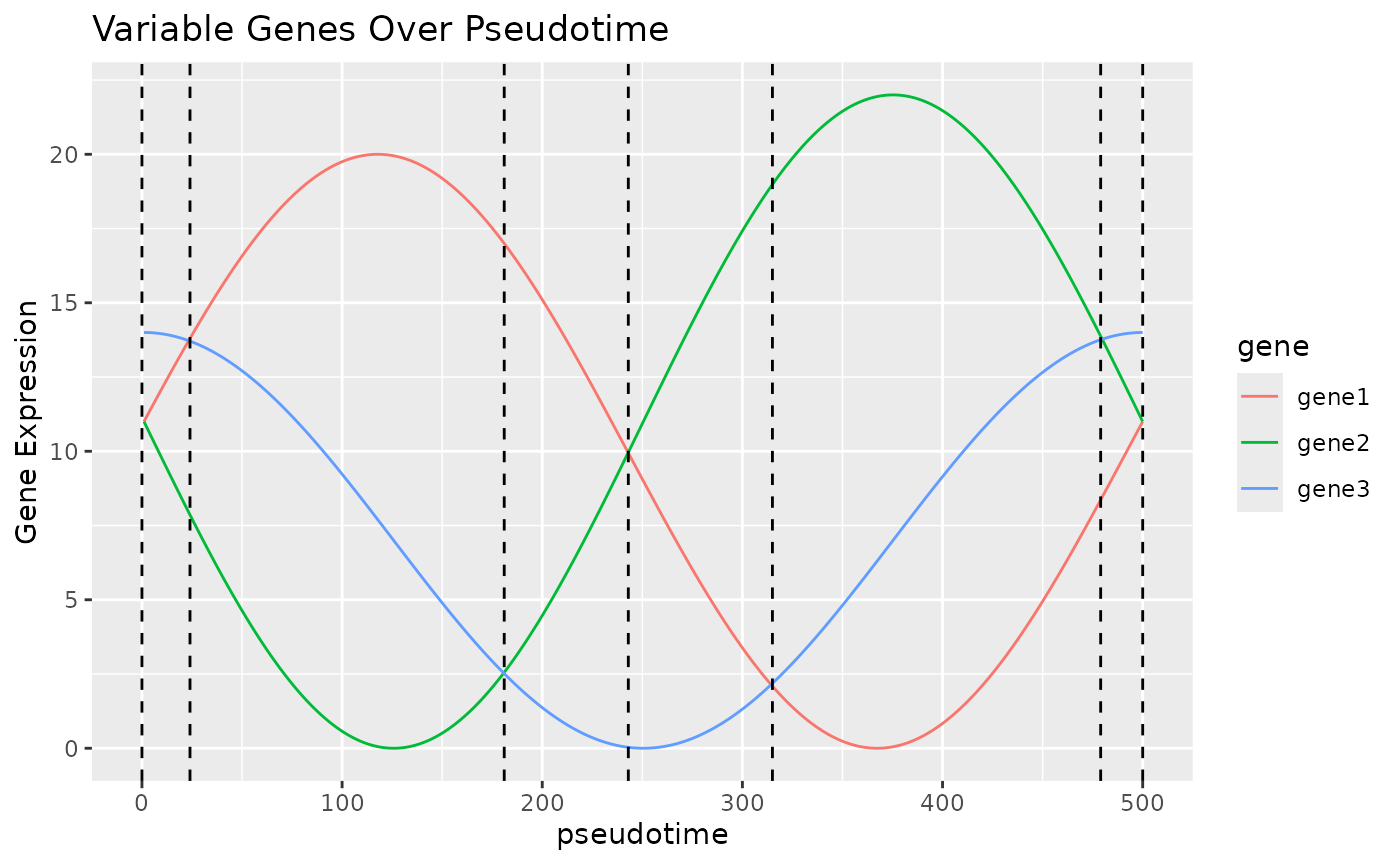
We believe that in many trajectories that cells undergo, there will be a curve that shows the expression of some key genes. In the plot below, we can see that by looking at these three “genes” which have 2 peaks each over “pseudotime”, we can identify 6 unique states, which, as long as the genes correspond to some aspect of the trajectory, can be used to infer which stage of the trajectory a cell is currently in. This is of course a constructed example and unlikely to be exactly repeated in real life, but hopefully demonstrates the principle BLASE works on.

# Adapted from
# https://codepal.ai/code-generator/query/n4dEA6I9/plot-sine-wave-ggplot2-r
x <- seq(0, 2 * pi, length.out = 500)
gene1_expr <- 10 * (sin(x + 0.1) + 1)
gene2_expr <- 11 * (sin(x - pi) + 1)
gene3_expr <- 7 * (sin(x + pi / 2) + 1)


genes <- data.frame(gene1 = gene1_expr, gene2 = gene2_expr, gene3 = gene3_expr)
genes_melt <- melt(t(genes), varnames = c("gene", "x"))
genes_melt$x <- as.numeric(genes_melt$x)

ggplot(genes_melt, aes = aes()) +
    geom_line(aes(x = x, y = value, color = gene)) +
    geom_vline(xintercept = 0, linetype = "dashed") +
    geom_vline(xintercept = 24, linetype = "dashed") +
    geom_vline(xintercept = 181, linetype = "dashed") +
    geom_vline(xintercept = 243, linetype = "dashed") +
    geom_vline(xintercept = 315, linetype = "dashed") +
    geom_vline(xintercept = 479, linetype = "dashed") +
    geom_vline(xintercept = 500, linetype = "dashed") +
    labs(
        x = "pseudotime",
        y = "Gene Expression",
        title = "Variable Genes Over Pseudotime"
    )

Plot showing gene expression varying over time for three genes, with lines marking different areas which can be uniquely identified by the rank-order of the expression of the genes.

Generating Icon

# Adapted from https://nelson-gon.github.io/12/06/2020/hex-sticker-creation-r/
library(fontawesome)
library(magick)
library(dplyr)
library(hexSticker)
library(devtools)

logo_color <- "orange"
fill_color <- "red"
border_color <- "red"

svg <- fa(name = "fire", fill = logo_color)

img <- image_read_svg(svg)
img %>%
    image_convert("png") %>%
    image_fill(color = fill_color, point = "+50") -> res

final_res <- sticker(res,
    package = "BLASE", p_size = 28,
    p_y = 1,
    s_x = 1, s_y = 1, s_width = 1.2,
    s_height = 14,
    filename = "blase_icon.png",
    h_fill = fill_color,
    h_color = border_color
)

plot(final_res)
usethis::use_logo("blase_icon.png")

Session Info

sessionInfo()
#> R version 4.5.1 (2025-06-13)
#> Platform: x86_64-pc-linux-gnu
#> Running under: Ubuntu 24.04.3 LTS
#> 
#> Matrix products: default
#> BLAS:   /usr/lib/x86_64-linux-gnu/openblas-pthread/libblas.so.3 
#> LAPACK: /usr/lib/x86_64-linux-gnu/openblas-pthread/libopenblasp-r0.3.26.so;  LAPACK version 3.12.0
#> 
#> locale:
#>  [1] LC_CTYPE=C.UTF-8       LC_NUMERIC=C           LC_TIME=C.UTF-8       
#>  [4] LC_COLLATE=C.UTF-8     LC_MONETARY=C.UTF-8    LC_MESSAGES=C.UTF-8   
#>  [7] LC_PAPER=C.UTF-8       LC_NAME=C              LC_ADDRESS=C          
#> [10] LC_TELEPHONE=C         LC_MEASUREMENT=C.UTF-8 LC_IDENTIFICATION=C   
#> 
#> time zone: UTC
#> tzcode source: system (glibc)
#> 
#> attached base packages:
#> [1] stats     graphics  grDevices utils     datasets  methods   base     
#> 
#> other attached packages:
#> [1] reshape2_1.4.4 ggplot2_3.5.2 
#> 
#> loaded via a namespace (and not attached):
#>  [1] gtable_0.3.6       jsonlite_2.0.0     dplyr_1.1.4        compiler_4.5.1    
#>  [5] tidyselect_1.2.1   Rcpp_1.1.0         stringr_1.5.1      jquerylib_0.1.4   
#>  [9] systemfonts_1.2.3  scales_1.4.0       textshaping_1.0.3  yaml_2.3.10       
#> [13] fastmap_1.2.0      R6_2.6.1           plyr_1.8.9         labeling_0.4.3    
#> [17] generics_0.1.4     knitr_1.50         htmlwidgets_1.6.4  tibble_3.3.0      
#> [21] desc_1.4.3         bslib_0.9.0        pillar_1.11.0      RColorBrewer_1.1-3
#> [25] rlang_1.1.6        stringi_1.8.7      cachem_1.1.0       xfun_0.53         
#> [29] fs_1.6.6           sass_0.4.10        cli_3.6.5          pkgdown_2.1.3     
#> [33] withr_3.0.2        magrittr_2.0.3     digest_0.6.37      grid_4.5.1        
#> [37] lifecycle_1.0.4    vctrs_0.6.5        evaluate_1.0.5     glue_1.8.0        
#> [41] farver_2.1.2       ragg_1.5.0         rmarkdown_2.29     tools_4.5.1       
#> [45] pkgconfig_2.0.3    htmltools_0.5.8.1