BLASE for excluding developmental genes from bulk RNA-seq
BLASE-for-excluding-developmental-genes-from-bulk-RNA-seq.Rmd
library(scater)
library(ggplot2)
library(BiocParallel)
library(blase)
library(limma)
library(ggVennDiagram)
RNGversion("3.5.0")
#> Warning in RNGkind("Mersenne-Twister", "Inversion", "Rounding"): non-uniform
#> 'Rounding' sampler used
SEED <- 7
set.seed(SEED)
N_CORES <- 2
bpparam <- MulticoreParam(N_CORES)
This article will show how BLASE can be used for excluding the effect of developmental differences when analysing bulk RNA-seq data. We make use of scRNA-seq Dogga et al. 2024 and bulk RNA-seq data from Zhang et al. 2021. Code for generating the objects used here is available in the BLASE reproducibility repository.
Load Data
First we’ll load in the data we’re using, pre-prepared from the BLASE reproducibility repository.
We can examine the true lifecycle stages, and also the calculated pseudotime trajectory (Slingshot).
plotUMAP(MCA_PF_SCE, colour_by = "STAGE_HR")
#| fig.alt: >
#| UMAP of Dogga et al. single-cell RNA-seq reference coloured by pseudotime,
#| starting with Rings, and ending with Schizonts.
plotUMAP(MCA_PF_SCE, colour_by = "slingPseudotime_1")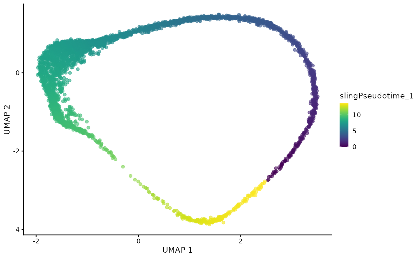 ## Prepare BLASE
Now we’ll prepare BLASE for use.
Create BLASE data object
First, we create the object, giving it the number of bins we want to use, and how to calculate them.
blase_data <- as.BlaseData(
    MCA_PF_SCE,
    pseudotime_slot = "slingPseudotime_1",
    n_bins = 8,
    split_by = "pseudotime_range"
)

# Add these bins to the sc metadata
MCA_PF_SCE <- assign_pseudotime_bins(MCA_PF_SCE,
    pseudotime_slot = "slingPseudotime_1",
    n_bins = 8,
    split_by = "pseudotime_range"
)
Select Genes
Now we will select the genes we want to use, using BLASE’s gene peakedness metric.
gene_peakedness_info <- calculate_gene_peakedness(
    MCA_PF_SCE,
    window_pct = 5,
    knots = 18,
    BPPARAM = bpparam
)

genes_to_use <- gene_peakedness_spread_selection(
    MCA_PF_SCE,
    gene_peakedness_info,
    genes_per_bin = 30,
    n_gene_bins = 30
)

head(gene_peakedness_info)
#>             gene peak_pseudotime mean_in_window mean_out_window     ratio
#> 28 PF3D7-1401100       3.8311312       5.793085        1.528934  3.788969
#> 44 PF3D7-1401200       6.0203490       4.791942        1.921439  2.493934
#> 29 PF3D7-1401400       3.9679573     696.174509       39.689901 17.540344
#> 84 PF3D7-1401600      11.4933936      93.076303        7.631160 12.196875
#> 1  PF3D7-1401900       0.1368261      43.270750        3.321464 13.027613
#> 80 PF3D7-1402200      10.9460892       3.754015        1.554102  2.415553
#>    window_start window_end deviance_explained
#> 28    3.4890659  4.1731965          0.1881312
#> 44    5.6782838  6.3624143          0.2035355
#> 29    3.6258920  4.3100226          0.2513795
#> 84   11.1513283 11.8354589          0.6891177
#> 1    -0.2052392  0.4788914          0.3846938
#> 80   10.6040239 11.2881544          0.1768597
Here, we add them to the BLASE object for mapping with.
genes(blase_data) <- genes_to_useCalculate Mappings
Now we can perform the actual mapping step, and review the results.
mapping_results <- map_all_best_bins(
    blase_data,
    zhang_2021_heat_shock_bulk,
    BPPARAM = bpparam
)
plot_mapping_result_heatmap(mapping_results)
#> Inferred correlation metric.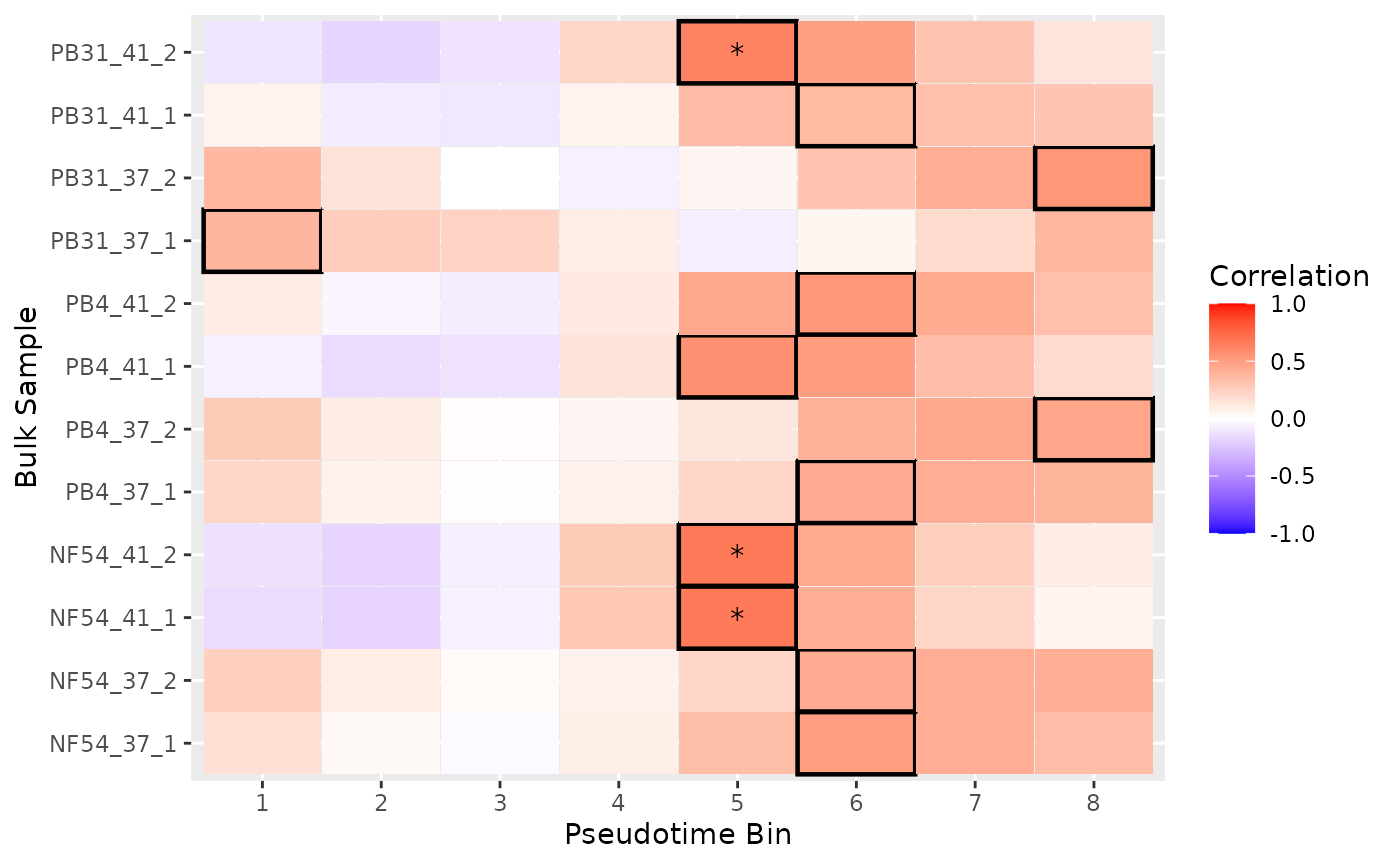
Calculate DE genes
We calculate DE genes using Limma (ref) as we have access to only normalised counts.
metadata <- data.frame(row.names = seq_len(12))
metadata$strain <- c(
    rep("NF54", 4),
    rep("PB4", 4),
    rep("PB31", 4)
)
metadata$growth_conditions <- rep(c("Normal", "Normal", "HS", "HS"), 3)
metadata$group <- paste0(metadata$strain, "_", metadata$growth_conditions)
rownames(metadata) <- c(
    "NF54_37_1",
    "NF54_37_2",
    "NF54_41_1",
    "NF54_41_2",
    "PB4_37_1",
    "PB4_37_2",
    "PB4_41_1",
    "PB4_41_2",
    "PB31_37_1",
    "PB31_37_2",
    "PB31_41_1",
    "PB31_41_2"
)

design <- model.matrix(~ 0 + group, metadata)
colnames(design) <- gsub("group", "", colnames(design))

contr.matrix <- makeContrasts(
    WT_normal_v_HS = NF54_Normal - NF54_HS,
    PB31_normal_v_HS = PB31_Normal - PB31_HS,
    normal_NF54_v_PB31 = NF54_Normal - PB31_Normal,
    levels = colnames(design)
)
Phenotype + Development (Bulk DE)
vfit <- lmFit(zhang_2021_heat_shock_bulk, design)
vfit <- contrasts.fit(vfit, contrasts = contr.matrix)
efit <- eBayes(vfit)

summary(decideTests(efit))
#>        WT_normal_v_HS PB31_normal_v_HS normal_NF54_v_PB31
#> Down              118              118                179
#> NotSig            822              616                767
#> Up                 50              256                 44

PB31_normal_v_HS_BULK_DE <- topTable(efit, n = Inf, coef = 2)
PB31_normal_v_HS_BULK_DE <- PB31_normal_v_HS_BULK_DE[
  PB31_normal_v_HS_BULK_DE$adj.P.Val < 0.05 &
    PB31_normal_v_HS_BULK_DE$logFC > 0, ]
PB31_normal_v_HS_BULK_DE <- PB31_normal_v_HS_BULK_DE[
  order(-PB31_normal_v_HS_BULK_DE$logFC), ]
Development (SC DE)
First, let’s pseudobulk based on the pseudotime bins
pseudobulked_MCA_PF_SCE <- data.frame(row.names = rownames(MCA_PF_SCE))
for (r in mapping_results) {
    pseudobulked_MCA_PF_SCE[bulk_name(r)] <- rowSums(
      counts(MCA_PF_SCE[, MCA_PF_SCE$pseudotime_bin == best_bin(r)]))
}
pseudobulked_MCA_PF_SCE <- as.matrix(pseudobulked_MCA_PF_SCE)
And now calculate DE genes for these
## Normalise, not needed for true bulks
par(mfrow = c(1, 2))
v <- voom(pseudobulked_MCA_PF_SCE, design, plot = FALSE)

vfit_sc <- lmFit(v, design)
vfit_sc <- contrasts.fit(vfit_sc, contrasts = contr.matrix)
efit_sc <- eBayes(vfit_sc)

summary(decideTests(efit_sc))
#>        WT_normal_v_HS PB31_normal_v_HS normal_NF54_v_PB31
#> Down                0              257                127
#> NotSig           1746             1370               1343
#> Up 0 119 276Remove Developmental Genes
How many of these genes overlap? We can look at the intersection using a Venn Diagram:
ggVennDiagram(list(
    Phenotype = rownames(PB31_normal_v_HS_BULK_DE),
    Development = rownames(PB31_normal_v_HS_SC_DE)
)) + ggtitle("PB31 Normal vs Heat Shock")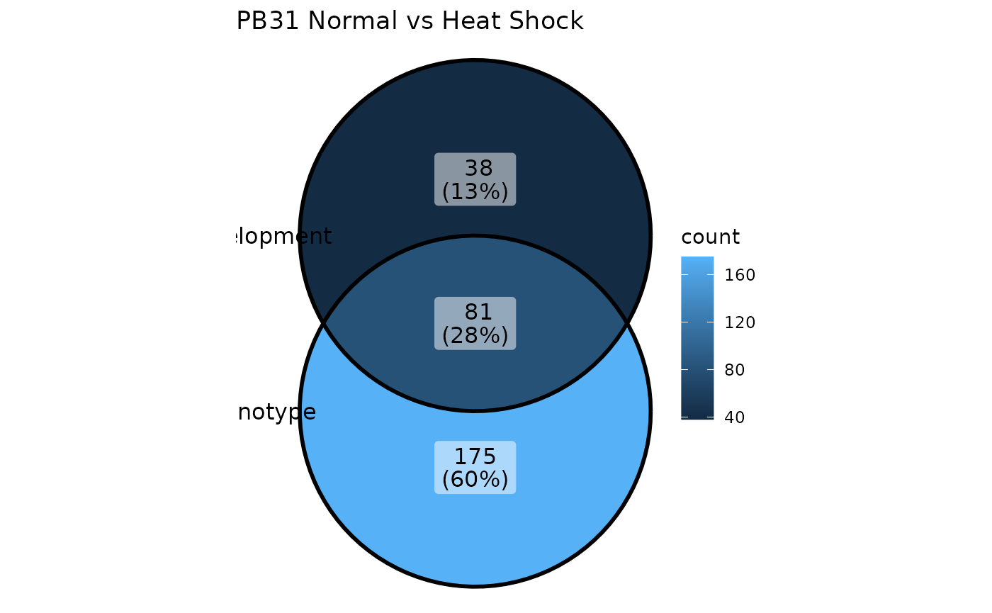
Great, there are genes which we can correct. We can now remove these from the original DE genes list.
NB: This is a primitive approach, and there are likely many other and better ways to calculate which genes should be kept or removed.
PB31_normal_v_HS_corrected_DE <- rownames(PB31_normal_v_HS_BULK_DE[
  !(rownames(PB31_normal_v_HS_BULK_DE) %in% rownames(PB31_normal_v_HS_SC_DE)),])
head(PB31_normal_v_HS_corrected_DE)
#> [1] "PF3D7-0725400" "PF3D7-0905400" "PF3D7-1010300" "PF3D7-0731500"
#> [5] "PF3D7-0913800" "PF3D7-1017500"
Further downstream analysis can now be performed, as desired by the researcher, for example Gene Ontology term enrichment.
Session Info
sessionInfo()
#> R version 4.6.0 (2026-04-24)
#> Platform: x86_64-pc-linux-gnu
#> Running under: Ubuntu 24.04.4 LTS
#>
#> Matrix products: default
#> BLAS:   /usr/lib/x86_64-linux-gnu/openblas-pthread/libblas.so.3
#> LAPACK: /usr/lib/x86_64-linux-gnu/openblas-pthread/libopenblasp-r0.3.26.so;  LAPACK version 3.12.0
#>
#> Random number generation:
#>  RNG:     Mersenne-Twister
#>  Normal:  Inversion
#>  Sample:  Rounding
#>
#> locale:
#>  [1] LC_CTYPE=C.UTF-8       LC_NUMERIC=C           LC_TIME=C.UTF-8
#>  [4] LC_COLLATE=C.UTF-8     LC_MONETARY=C.UTF-8    LC_MESSAGES=C.UTF-8
#>  [7] LC_PAPER=C.UTF-8       LC_NAME=C              LC_ADDRESS=C
#> [10] LC_TELEPHONE=C         LC_MEASUREMENT=C.UTF-8 LC_IDENTIFICATION=C
#>
#> time zone: UTC
#> tzcode source: system (glibc)
#>
#> attached base packages:
#> [1] stats4    stats     graphics  grDevices utils     datasets  methods
#> [8] base
#>
#> other attached packages:
#>  [1] ggVennDiagram_1.5.7         limma_3.68.3
#>  [3] blase_1.3.0                 BiocParallel_1.46.0
#>  [5] scater_1.40.1               ggplot2_4.0.3
#>  [7] scuttle_1.22.0              SingleCellExperiment_1.34.0
#>  [9] SummarizedExperiment_1.42.0 Biobase_2.72.0
#> [11] GenomicRanges_1.64.0        Seqinfo_1.2.0
#> [13] IRanges_2.46.0              S4Vectors_0.50.1
#> [15] BiocGenerics_0.58.1         generics_0.1.4
#> [17] MatrixGenerics_1.24.0       matrixStats_1.5.0
#> [19] BiocStyle_2.40.0
#>
#> loaded via a namespace (and not attached):
#>   [1] RcppAnnoy_0.0.23         splines_4.6.0            later_1.4.8
#>   [4] tibble_3.3.1             polyclip_1.10-7          fastDummies_1.7.6
#>   [7] lifecycle_1.0.5          globals_0.19.1           lattice_0.22-9
#>  [10] MASS_7.3-65              SnowballC_0.7.1          magrittr_2.0.5
#>  [13] plotly_4.12.0            sass_0.4.10              rmarkdown_2.31
#>  [16] jquerylib_0.1.4          yaml_2.3.12              httpuv_1.6.17
#>  [19] otel_0.2.0               Seurat_5.5.0             sctransform_0.4.3
#>  [22] spam_2.11-3              sp_2.2-1                 spatstat.sparse_3.2-0
#>  [25] reticulate_1.46.0        cowplot_1.2.0            pbapply_1.7-4
#>  [28] RColorBrewer_1.1-3       abind_1.4-8              Rtsne_0.17
#>  [31] purrr_1.2.2              ggrepel_0.9.8            irlba_2.3.7
#>  [34] listenv_0.10.1           spatstat.utils_3.2-3     goftest_1.2-3
#>  [37] RSpectra_0.16-2          spatstat.random_3.5-0    fitdistrplus_1.2-6
#>  [40] parallelly_1.47.0        pkgdown_2.2.0            codetools_0.2-20
#>  [43] DelayedArray_0.38.1      tidyselect_1.2.1         farver_2.1.2
#>  [46] ScaledMatrix_1.20.0      viridis_0.6.5            spatstat.explore_3.8-1
#>  [49] jsonlite_2.0.0           BiocNeighbors_2.6.0      progressr_0.19.0
#>  [52] ggridges_0.5.7           survival_3.8-6           systemfonts_1.3.2
#>  [55] tools_4.6.0              ragg_1.5.2               ica_1.0-3
#>  [58] Rcpp_1.1.1-1.1           glue_1.8.1               gridExtra_2.3
#>  [61] SparseArray_1.12.2       xfun_0.57                mgcv_1.9-4
#>  [64] dplyr_1.2.1              withr_3.0.2              BiocManager_1.30.27
#>  [67] fastmap_1.2.0            boot_1.3-32              digest_0.6.39
#>  [70] rsvd_1.0.5               R6_2.6.1                 mime_0.13
#>  [73] textshaping_1.0.5        scattermore_1.2          tensor_1.5.1
#>  [76] spatstat.data_3.1-9      tidyr_1.3.2              data.table_1.18.4
#>  [79] httr_1.4.8               htmlwidgets_1.6.4        S4Arrays_1.12.0
#>  [82] uwot_0.2.4               pkgconfig_2.0.3          gtable_0.3.6
#>  [85] lmtest_0.9-40            S7_0.2.2                 XVector_0.52.0
#>  [88] htmltools_0.5.9          dotCall64_1.2            bookdown_0.46
#>  [91] SeuratObject_5.4.0       scales_1.4.0             png_0.1-9
#>  [94] spatstat.univar_3.2-0    knitr_1.51               reshape2_1.4.5
#>  [97] nlme_3.1-169             cachem_1.1.0             zoo_1.8-15
#> [100] stringr_1.6.0            KernSmooth_2.23-26       parallel_4.6.0
#> [103] miniUI_0.1.2             vipor_0.4.7              desc_1.4.3
#> [106] pillar_1.11.1            grid_4.6.0               vctrs_0.7.3
#> [109] RANN_2.6.2               lsa_0.73.4               promises_1.5.0
#> [112] BiocSingular_1.28.0      beachmat_2.28.0          xtable_1.8-8
#> [115] cluster_2.1.8.2          beeswarm_0.4.0           evaluate_1.0.5
#> [118] cli_3.6.6                compiler_4.6.0           rlang_1.2.0
#> [121] future.apply_1.20.2      labeling_0.4.3           plyr_1.8.9
#> [124] fs_2.1.0                 ggbeeswarm_0.7.3         stringi_1.8.7
#> [127] viridisLite_0.4.3        deldir_2.0-4             lazyeval_0.2.3
#> [130] spatstat.geom_3.8-1      Matrix_1.7-5             RcppHNSW_0.6.0
#> [133] patchwork_1.3.2          sparseMatrixStats_1.24.0 future_1.70.0
#> [136] statmod_1.5.2            shiny_1.13.0             ROCR_1.0-12
#> [139] igraph_2.3.1             bslib_0.11.0