BLASE for annotating scRNA-seq • blase

library(scater)
library(ggplot2)
library(BiocParallel)
library(blase)
library(patchwork)

RNGversion("3.5.0")
#> Warning in RNGkind("Mersenne-Twister", "Inversion", "Rounding"): non-uniform
#> 'Rounding' sampler used
SEED <- 7
set.seed(SEED)

N_CORES <- 4
if (ami::using_ci()) {
    N_CORES <- 2
}
bpparam <- MulticoreParam(N_CORES)

This article will show how BLASE can be used for annotating scRNA-seq data using existing bulk or microarray data. We make use of scRNA-seq Dogga et al. 2024 and microarray data from Painter et al. 2018. Code for generating the objects used here is available in the BLASE reproducibility repository.

Load Data

First we’ll load in the data we’re using, pre-prepared from the BLASE reproducibility repository.

painter_microarray <- readRDS("Data/painter_2018_pf.rds")
dogga_sc <- readRDS("Data/MCA_PF_SCE.rds")

We can examine the true lifecycle stages, and also the calculated pseudotime trajectory (Slingshot).

plotUMAP(dogga_sc, colour_by = "STAGE_HR")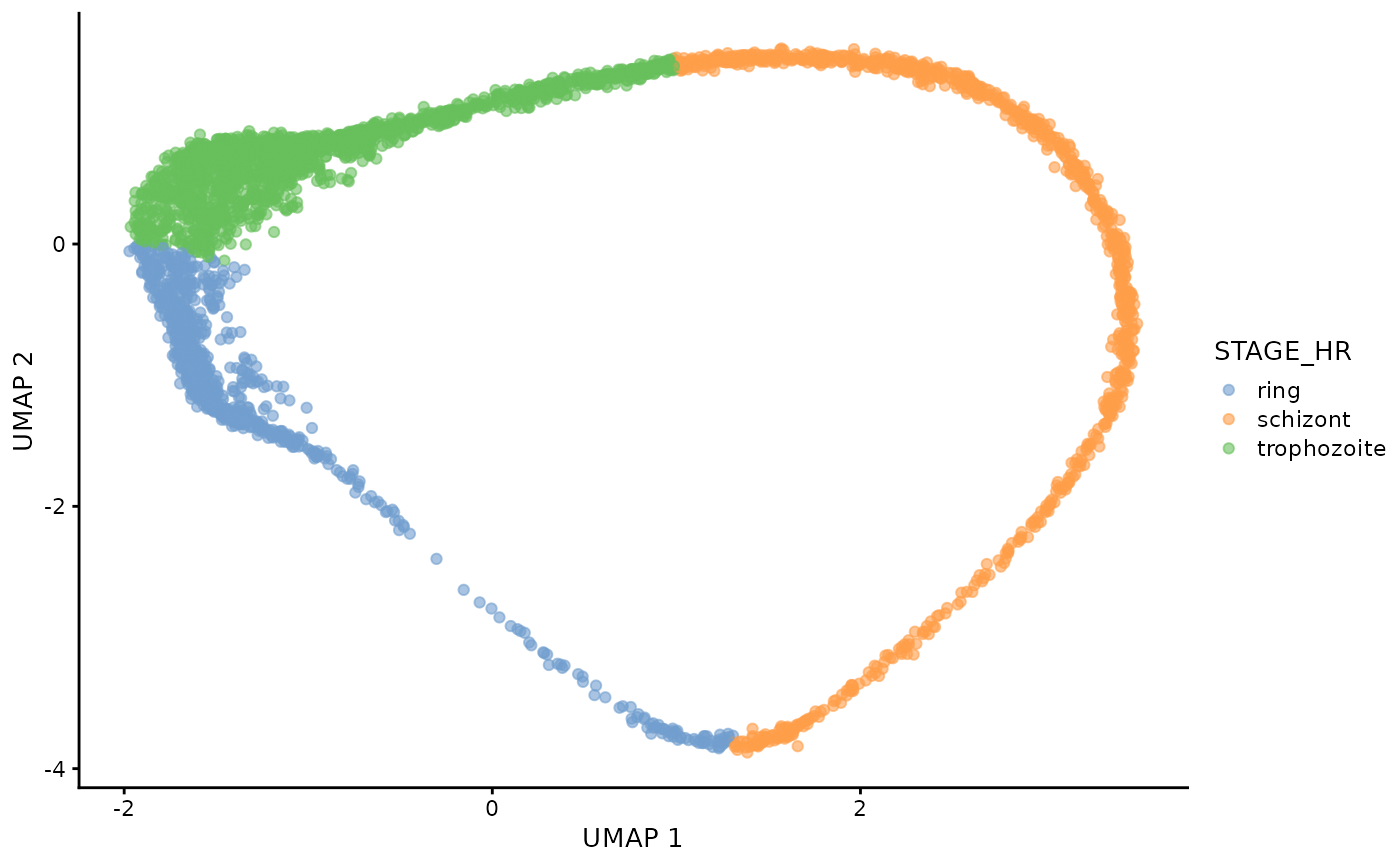

UMAP of Dogga et al. single-cell RNA-seq reference coloured by lifecycle stage, showing the cycle from Rings, Trophozoites, Schizonts, to Rings again.

#| fig.alt: >
#|   UMAP of Dogga et al. single-cell RNA-seq reference coloured by pseudotime,
#|   starting with Rings, and ending with Schizonts.
plotUMAP(dogga_sc, colour_by = "slingPseudotime_1")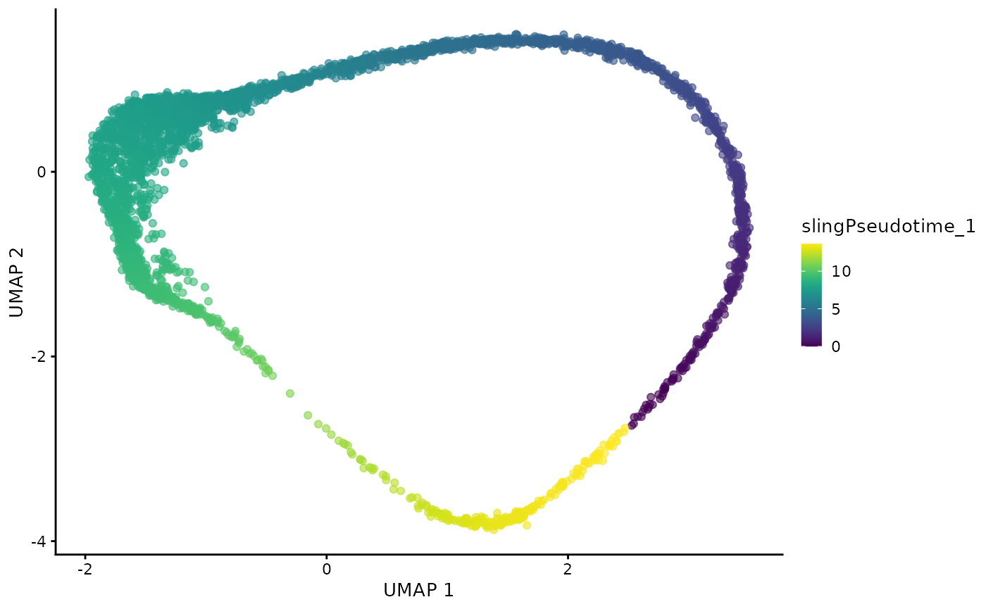

UMAP of Dogga et al. single-cell RNA-seq reference coloured by lifecycle stage, showing the cycle from Rings, Trophozoites, Schizonts, to Rings again.

Prepare BLASE

Now we’ll prepare BLASE for use.

Create BLASE data object

First, we create the object, giving it the number of bins we want to use, and how to calculate them.

blase_data <- as.BlaseData(
    dogga_sc,
    pseudotime_slot = "slingPseudotime_1",
    n_bins = 48,
    split_by = "cells"
)

# Add these bins to the sc metadata
dogga_sc <- blase::assign_pseudotime_bins(dogga_sc,
    pseudotime_slot = "slingPseudotime_1",
    n_bins = 48,
    split_by = "cells"
)

Select Genes

Now we will select the genes we want to use, using BLASE’s gene peakedness metric.

gene_peakedness_info <- blase::calculate_gene_peakedness(
    dogga_sc,
    window_pct = 5,
    knots = 18,
    BPPARAM = bpparam
)

genes_to_use <- blase::gene_peakedness_spread_selection(
    dogga_sc,
    gene_peakedness_info,
    genes_per_bin = 30,
    n_gene_bins = 30
)

head(gene_peakedness_info)
#>              gene peak_pseudotime mean_in_window mean_out_window     ratio
#> 72  PF3D7-1401100        9.811180       5.946666        1.576877  3.771165
#> 57  PF3D7-1401200        7.767184       4.928158        1.981323  2.487307
#> 59  PF3D7-1401300        8.039717       2.207782        1.285688  1.717199
#> 721 PF3D7-1401400        9.811180     942.073177       49.944485 18.862406
#> 15  PF3D7-1401600        2.043996      96.706165        8.207937 11.782031
#> 19  PF3D7-1402200        2.589061       3.516862        1.549402  2.269819
#>     window_start window_end deviance_explained
#> 72      9.470514  10.151846         0.16478147
#> 57      7.426518   8.107850         0.19846899
#> 59      7.699051   8.380383         0.04479178
#> 721     9.470514  10.151846         0.27186813
#> 15      1.703330   2.384662         0.64855890
#> 19      2.248395   2.929727         0.17093181

By using the gene_peakedness_spread_selection function, we can ensure that genes with high ratios are selected from throughout the trajectory.

ggplot(gene_peakedness_info, aes(x = peak_pseudotime, y = ratio)) +
    geom_point() +
    ggtitle("All genes")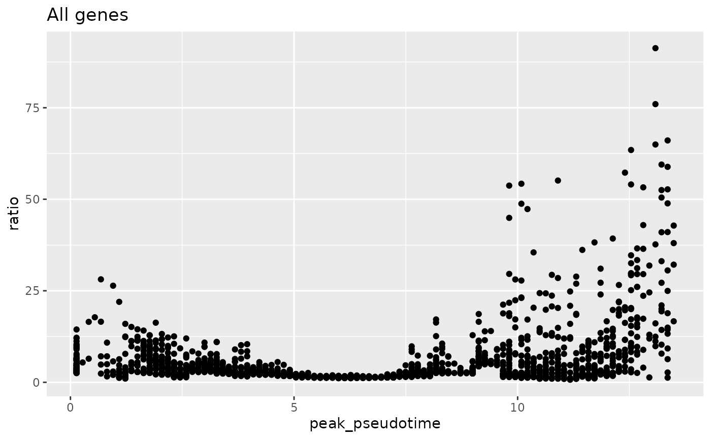

Scatter plot showing gene peakedness ratios for all genes, ordered by pseudotime.


gene_peakedness_selected_genes <- gene_peakedness_info[
    gene_peakedness_info$gene %in% genes_to_use,
]

ggplot(gene_peakedness_selected_genes, aes(x = peak_pseudotime, y = ratio)) +
    geom_point() +
    ggtitle("Selected genes")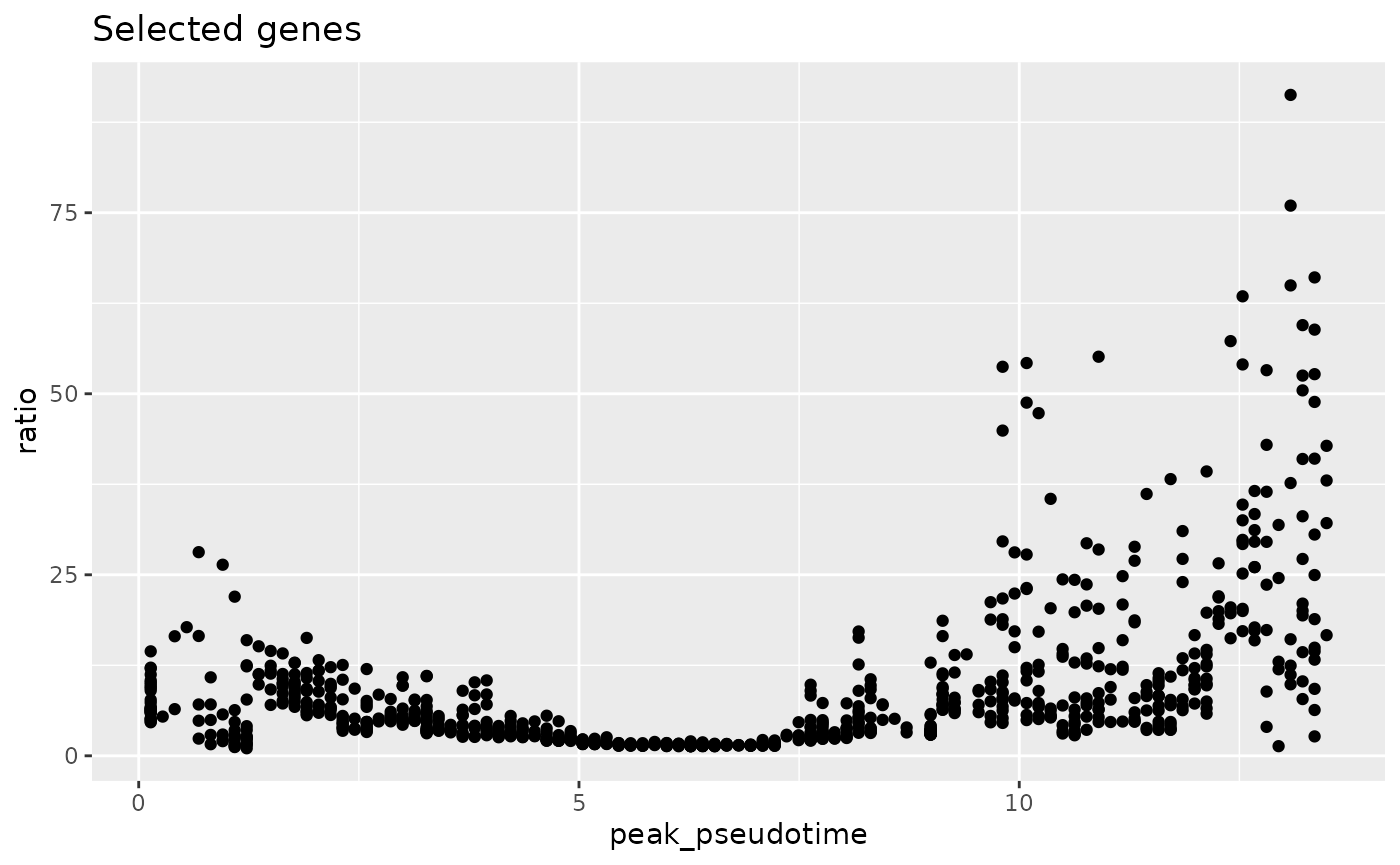

Scatter plot showing gene peakedness ratios for genes selected by BLASE spread selection, ordered by pseudotime.

Here, we add them to the BLASE object for mapping with.

genes(blase_data) <- genes_to_use

Calculate Mappings

Now we can perform the actual mapping step, and review the results.

mapping_results <- blase::map_all_best_bins(
    blase_data,
    painter_microarray,
    BPPARAM = bpparam
)

blase::plot_mapping_result_heatmap(mapping_results)

Heatmap of mapping correlations of the Painter et al. data onto the Dogga et al. scRNA-seq.

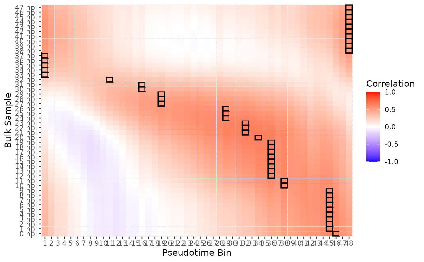
Transfer Mappings

In the Painter et al. paper, the expected lifecycle stages are as follows: | Lifecycle Stage | Painter et al. HPI | |—————–|——————–| | Ring | 0-21 | | Trophozoite | 16-32 | | Schizont | 33-48 |

We can use this to transfer back to the scRNA-seq as follows:

plotUMAP(dogga_sc, colour_by = "pseudotime_bin")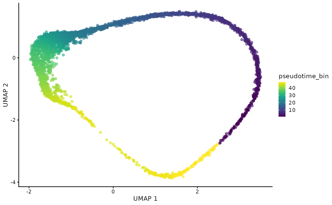

A UMAP of the reference scRNA-seq data coloured by pseudotime bin, as calculated by BLASE.

annotated_sce <- blase::annotate_sce(dogga_sc, mapping_results, include_stats = TRUE)
annotated_sce$BLASE_Annotation <- gsub(" hpi", "", annotated_sce$BLASE_Annotation)
annotated_sce$BLASE_Annotation <- as.numeric(annotated_sce$BLASE_Annotation)

annotation_plot <- plotUMAP(annotated_sce, colour_by = "BLASE_Annotation")
corr_plot <- plotUMAP(annotated_sce, colour_by = "BLASE_Annotation_Correlation") +
    labs(color = "Correlation")

annotation_plot + corr_plot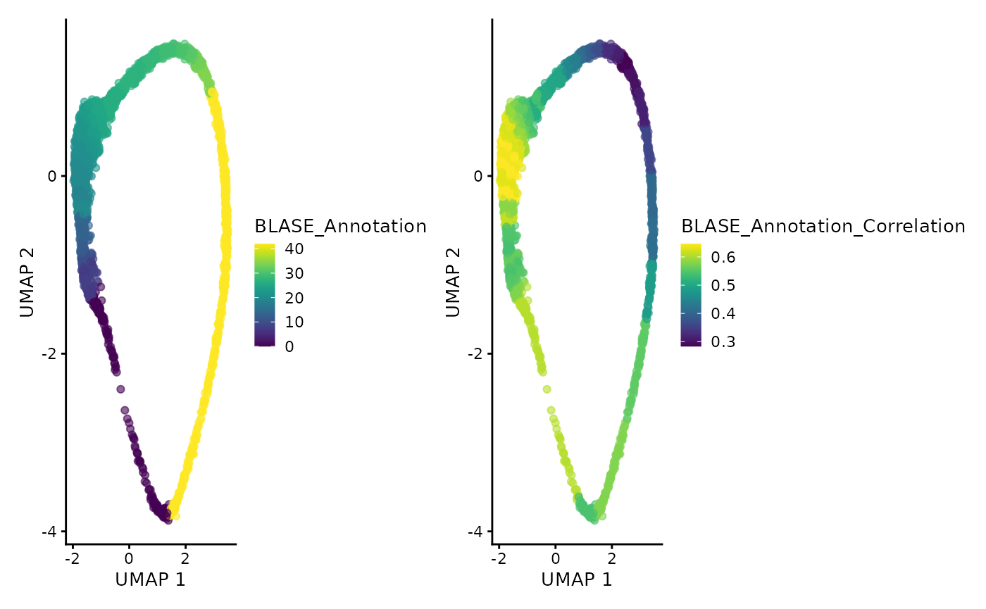

UMAP of Dogga et al. single-cell RNA-seq reference coloured by best matching bulk RNA-seq sample (hpi). Beside it is a UMAP of the correlations of these mappings.

annotated_sce$BLASE_Annotation_transfer <- ""
for (best_bulk in unique(annotated_sce$BLASE_Annotation)) {
    mask <- colData(annotated_sce)[, "BLASE_Annotation"] == best_bulk

    if (best_bulk %in% 0:15) {
        annotated_sce[, mask]$BLASE_Annotation_transfer <- "Ring"
    } else if (best_bulk %in% 16:21) {
        annotated_sce[, mask]$BLASE_Annotation_transfer <- "Ring/Trophozoite"
    } else if (best_bulk %in% 22:32) {
        annotated_sce[, mask]$BLASE_Annotation_transfer <- "Trophozoite"
    } else if (best_bulk %in% 33:48) {
        annotated_sce[, mask]$BLASE_Annotation_transfer <- "Schizont"
    }
}

plotUMAP(annotated_sce, colour_by = "BLASE_Annotation_transfer") +
    plotUMAP(annotated_sce, colour_by = "STAGE_LR")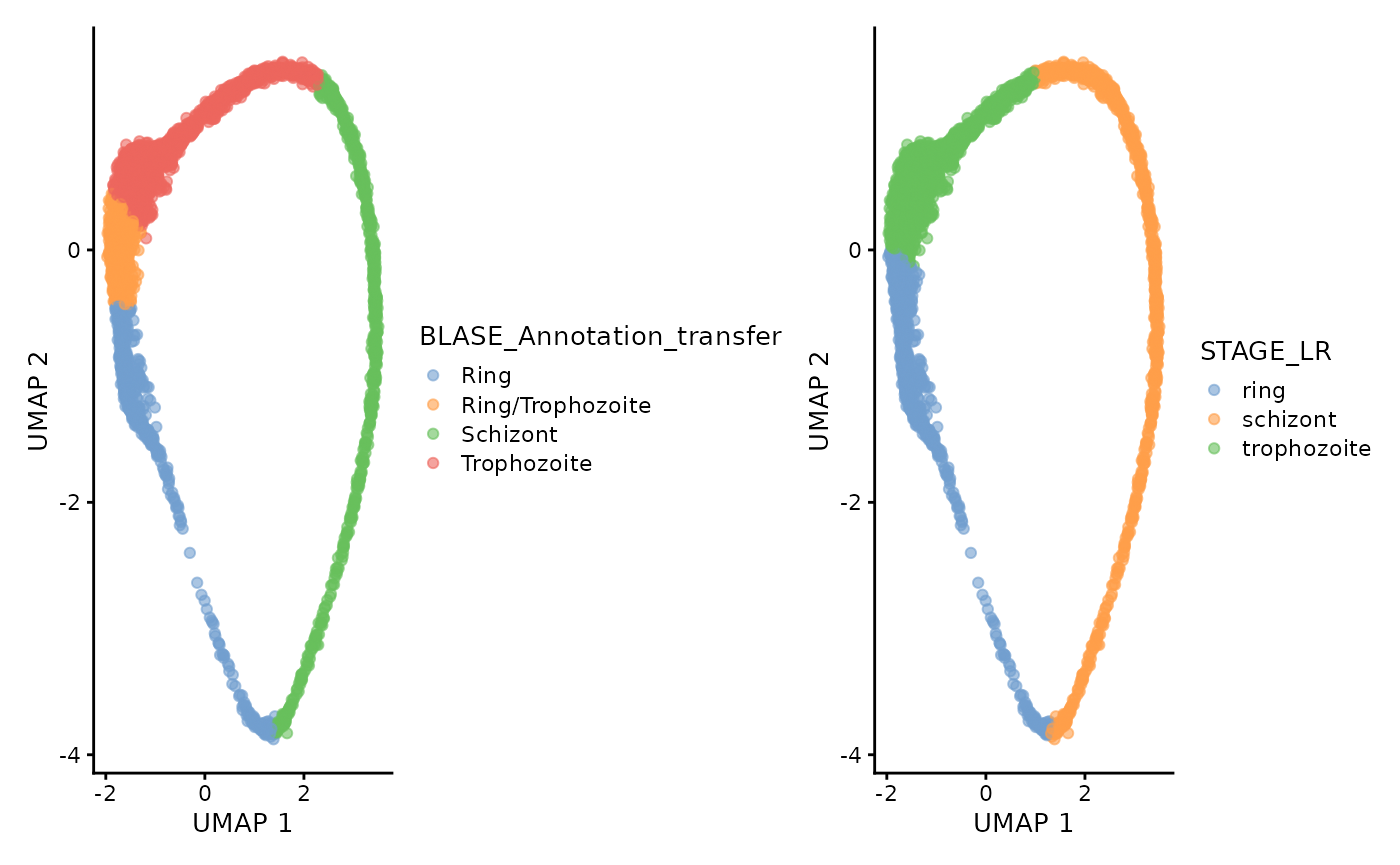

UMAP of Dogga et al. single-cell RNA-seq reference coloured the original mappings from Dogga et al. and by best matching bulk RNA-seq sample, and then named by the expected cell type ( from annotations in Painter et al.). The mappings are broadly the same.

Session Info

sessionInfo()
#> R version 4.5.1 (2025-06-13)
#> Platform: x86_64-pc-linux-gnu
#> Running under: Ubuntu 24.04.3 LTS
#> 
#> Matrix products: default
#> BLAS:   /usr/lib/x86_64-linux-gnu/openblas-pthread/libblas.so.3 
#> LAPACK: /usr/lib/x86_64-linux-gnu/openblas-pthread/libopenblasp-r0.3.26.so;  LAPACK version 3.12.0
#> 
#> Random number generation:
#>  RNG:     Mersenne-Twister 
#>  Normal:  Inversion 
#>  Sample:  Rounding 
#>  
#> locale:
#>  [1] LC_CTYPE=C.UTF-8       LC_NUMERIC=C           LC_TIME=C.UTF-8       
#>  [4] LC_COLLATE=C.UTF-8     LC_MONETARY=C.UTF-8    LC_MESSAGES=C.UTF-8   
#>  [7] LC_PAPER=C.UTF-8       LC_NAME=C              LC_ADDRESS=C          
#> [10] LC_TELEPHONE=C         LC_MEASUREMENT=C.UTF-8 LC_IDENTIFICATION=C   
#> 
#> time zone: UTC
#> tzcode source: system (glibc)
#> 
#> attached base packages:
#> [1] stats4    stats     graphics  grDevices utils     datasets  methods  
#> [8] base     
#> 
#> other attached packages:
#>  [1] patchwork_1.3.2             blase_0.99.0               
#>  [3] BiocParallel_1.42.1         scater_1.36.0              
#>  [5] ggplot2_3.5.2               scuttle_1.18.0             
#>  [7] SingleCellExperiment_1.30.1 SummarizedExperiment_1.38.1
#>  [9] Biobase_2.68.0              GenomicRanges_1.60.0       
#> [11] GenomeInfoDb_1.44.2         IRanges_2.42.0             
#> [13] S4Vectors_0.46.0            BiocGenerics_0.54.0        
#> [15] generics_0.1.4              MatrixGenerics_1.20.0      
#> [17] matrixStats_1.5.0          
#> 
#> loaded via a namespace (and not attached):
#>  [1] tidyselect_1.2.1         viridisLite_0.4.2        ami_0.2.1               
#>  [4] dplyr_1.1.4              vipor_0.4.7              farver_2.1.2            
#>  [7] viridis_0.6.5            fastmap_1.2.0            digest_0.6.37           
#> [10] rsvd_1.0.5               lifecycle_1.0.4          magrittr_2.0.3          
#> [13] compiler_4.5.1           rlang_1.1.6              sass_0.4.10             
#> [16] tools_4.5.1              yaml_2.3.10              knitr_1.50              
#> [19] labeling_0.4.3           S4Arrays_1.8.1           htmlwidgets_1.6.4       
#> [22] DelayedArray_0.34.1      RColorBrewer_1.1-3       abind_1.4-8             
#> [25] withr_3.0.2              desc_1.4.3               grid_4.5.1              
#> [28] beachmat_2.24.0          scales_1.4.0             cli_3.6.5               
#> [31] rmarkdown_2.29           crayon_1.5.3             ragg_1.5.0              
#> [34] httr_1.4.7               ggbeeswarm_0.7.2         cachem_1.1.0            
#> [37] splines_4.5.1            parallel_4.5.1           XVector_0.48.0          
#> [40] vctrs_0.6.5              boot_1.3-31              Matrix_1.7-3            
#> [43] jsonlite_2.0.0           BiocSingular_1.24.0      BiocNeighbors_2.2.0     
#> [46] ggrepel_0.9.6            irlba_2.3.5.1            beeswarm_0.4.0          
#> [49] systemfonts_1.2.3        jquerylib_0.1.4          glue_1.8.0              
#> [52] pkgdown_2.1.3            codetools_0.2-20         cowplot_1.2.0           
#> [55] gtable_0.3.6             UCSC.utils_1.4.0         ScaledMatrix_1.16.0     
#> [58] tibble_3.3.0             pillar_1.11.0            htmltools_0.5.8.1       
#> [61] GenomeInfoDbData_1.2.14  R6_2.6.1                 sparseMatrixStats_1.20.0
#> [64] textshaping_1.0.3        evaluate_1.0.5           lattice_0.22-7          
#> [67] bslib_0.9.0              Rcpp_1.1.0               gridExtra_2.3           
#> [70] SparseArray_1.8.1        nlme_3.1-168             mgcv_1.9-3              
#> [73] xfun_0.53                fs_1.6.6                 pkgconfig_2.0.3